Machine Learning: Supervised and Unsupervised

Introduction

This project was completed as part of my AI course, addressing two machine learning objectives. In the supervised learning component, I utilized Polynomial Ridge Regression to predict a target variable z based on input features x and y. For the unsupervised learning task, I applied Gaussian Mixture Models (GMM) to identify clusters within two datasets, labeled A and B. With a supervised dataset of 50 samples and two undisclosed datasets for unsupervised analysis, my goal was to develop effective models and present the outcomes through clear visualizations. This page outlines my methodology and findings.

---

How to Run It

Repo: SL-and-UL-machine-learning

Supervised Learning

• Dependencies:

  pip install scikit-learn numpy pandas
  

• Steps:
  1. Clone the repo.
  2. To train a model: python3 train_model.py
  3. To visualize results: python3 visualize_model.py
• Other useful scripts
  1. Generate synthetic data: python3 generate_samples.py
  2. Plot x and y vs. z: python3 xy.py

Unsupervised Learning

• Done in MATLAB. Needs datasets A and B (not shared here). Run the script to fit GMMs and see cluster plots.

---

Supervised Learning: Polynomial Ridge Regression

Task

I was provided with three CSV files: x and y as input attributes and z as the target variable. Each contains 50 float values in a single row. The task was to select a supervised learning method, train multiple models, and predict z for unseen data, outputting the results to z-predicted.csv.

Approach

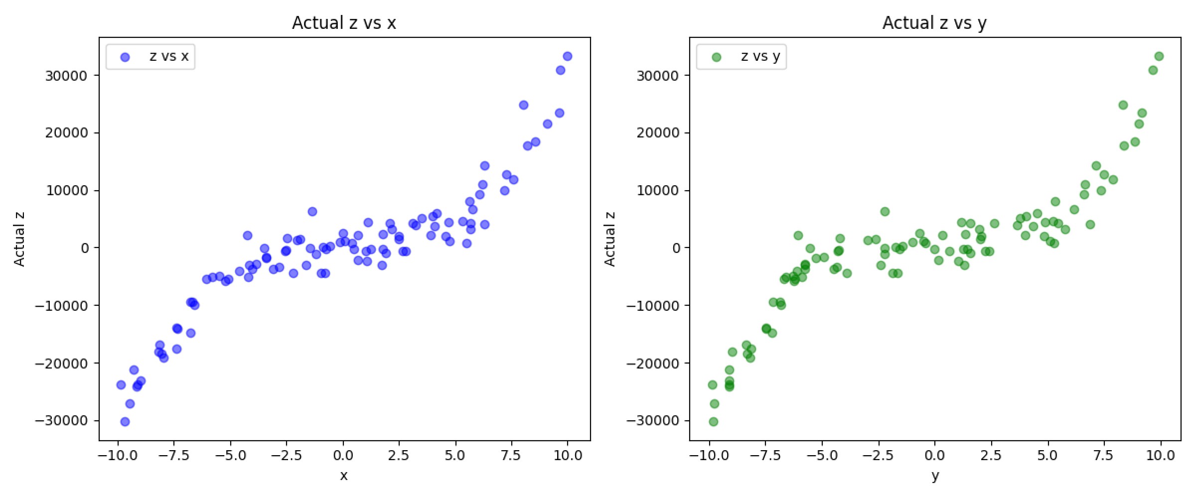
I first wanted to visualize what I was working with to see if there were any trends or patterns I could identify. I stacked x and y into a 50x2 matrix and plotted them against z with a quick matplotlib script:

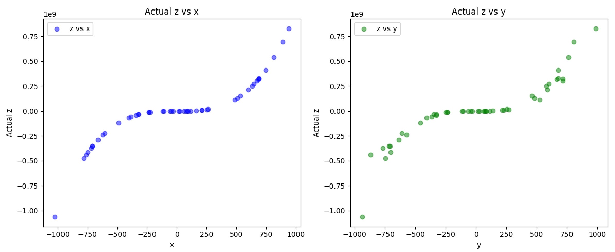
Immediately what stood out to me was that this data was non-linear and followed a cubic trend. This meant I could use Polynomial Regression to follow the polynomial function. Because it’s cubic, that means I would use a degree 3 to match the curve. But there’s also slight noise in the data, and a plain linear regressor would risk overfitting. So we need a way to regularize against this. This is when I discovered Ridge Regression, but first to demonstrate, here is an example of a trained model that utilizes a linear regressor (alpha=0, no regularization):

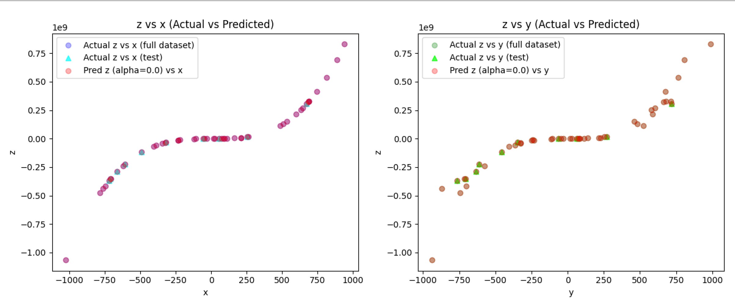
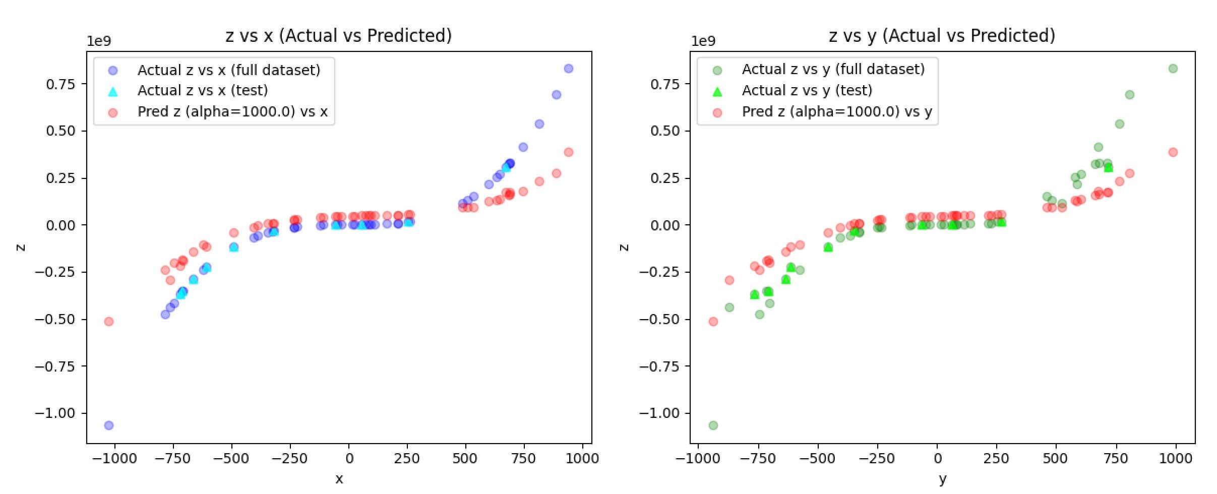
The predicted z values (red) align exactly with the original data which is a clear sign of severe overfitting. This is where ridge regression can come in to smooth out the predictions and more closely follow an underlining trend. Ridge adds an L2 penalty via an alpha constant. A higher alpha means more noise control. I ran a couple more tests to find an optimal alpha constant [10, 25, 100, 1000]:

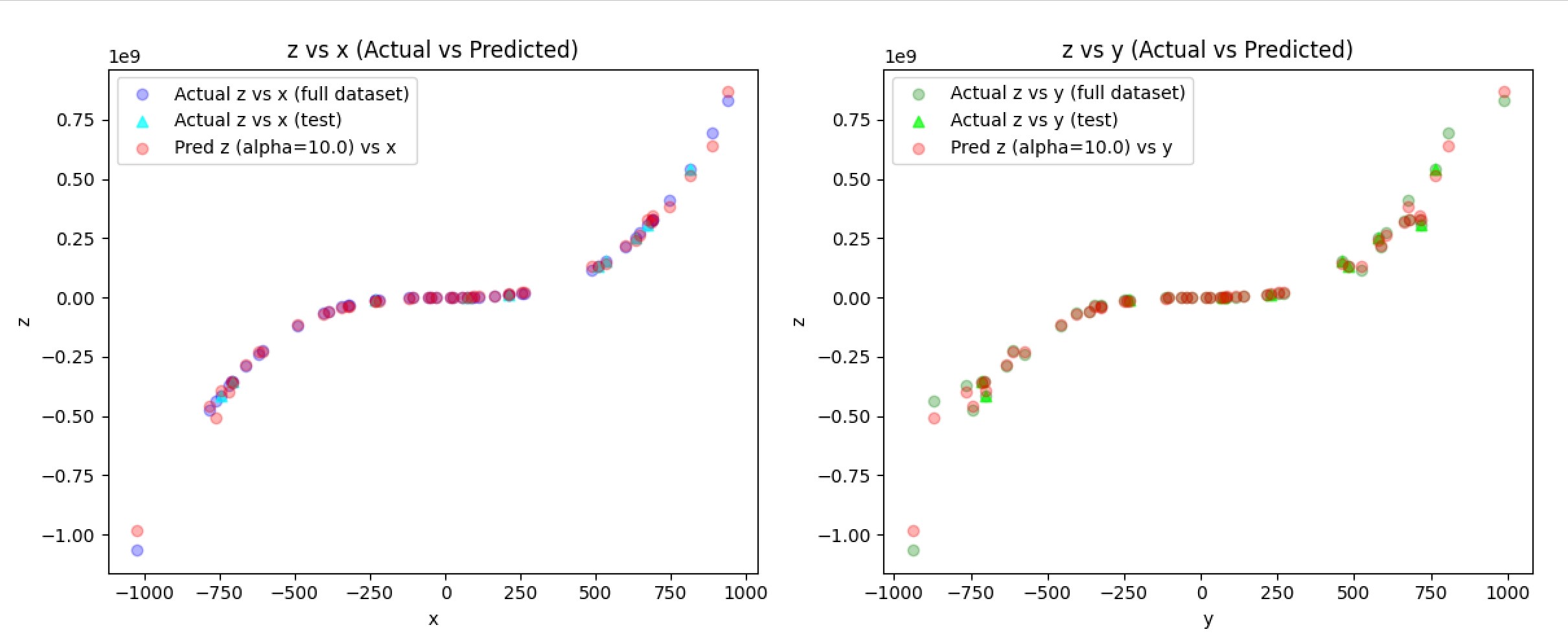
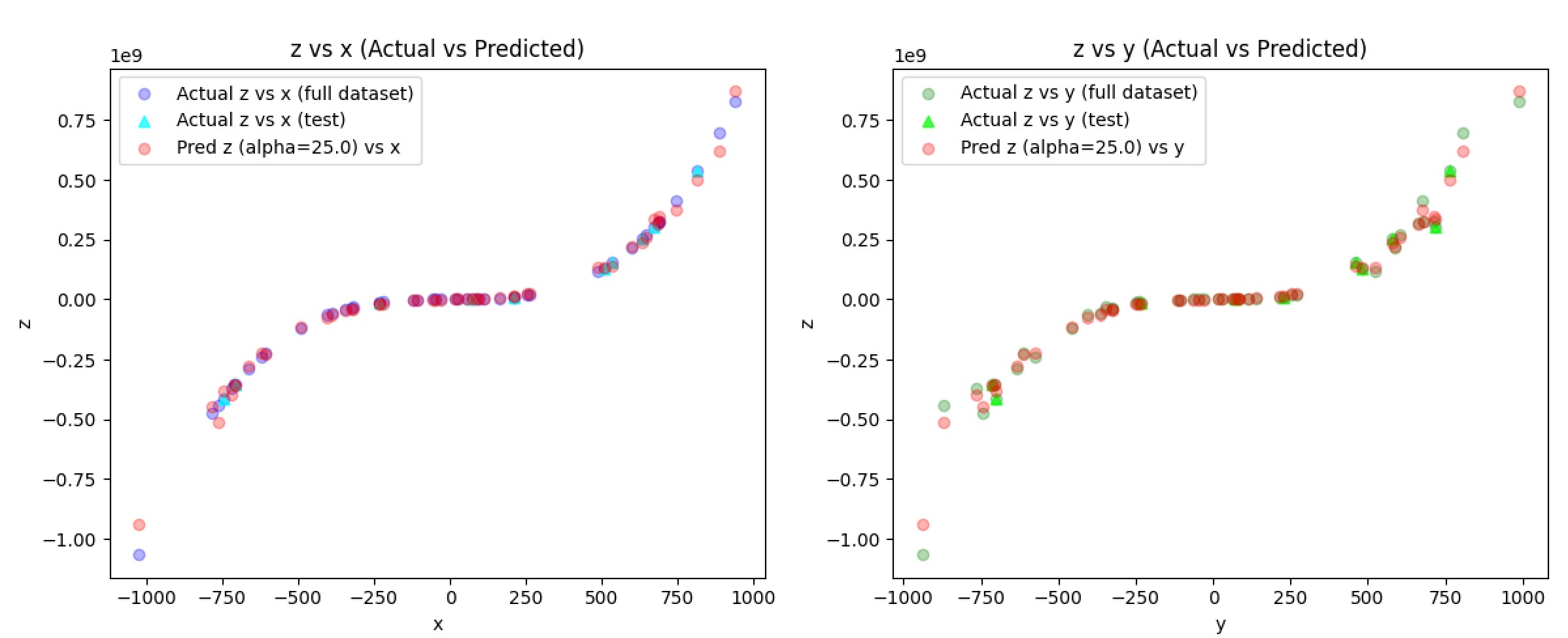
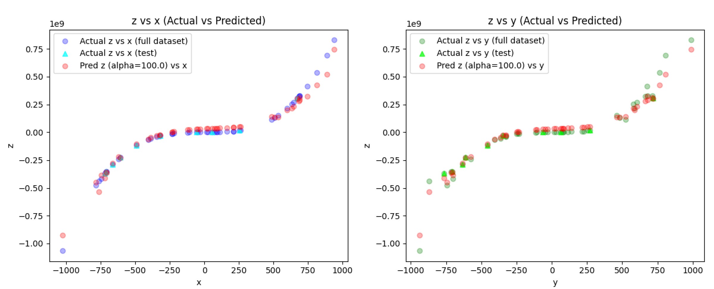
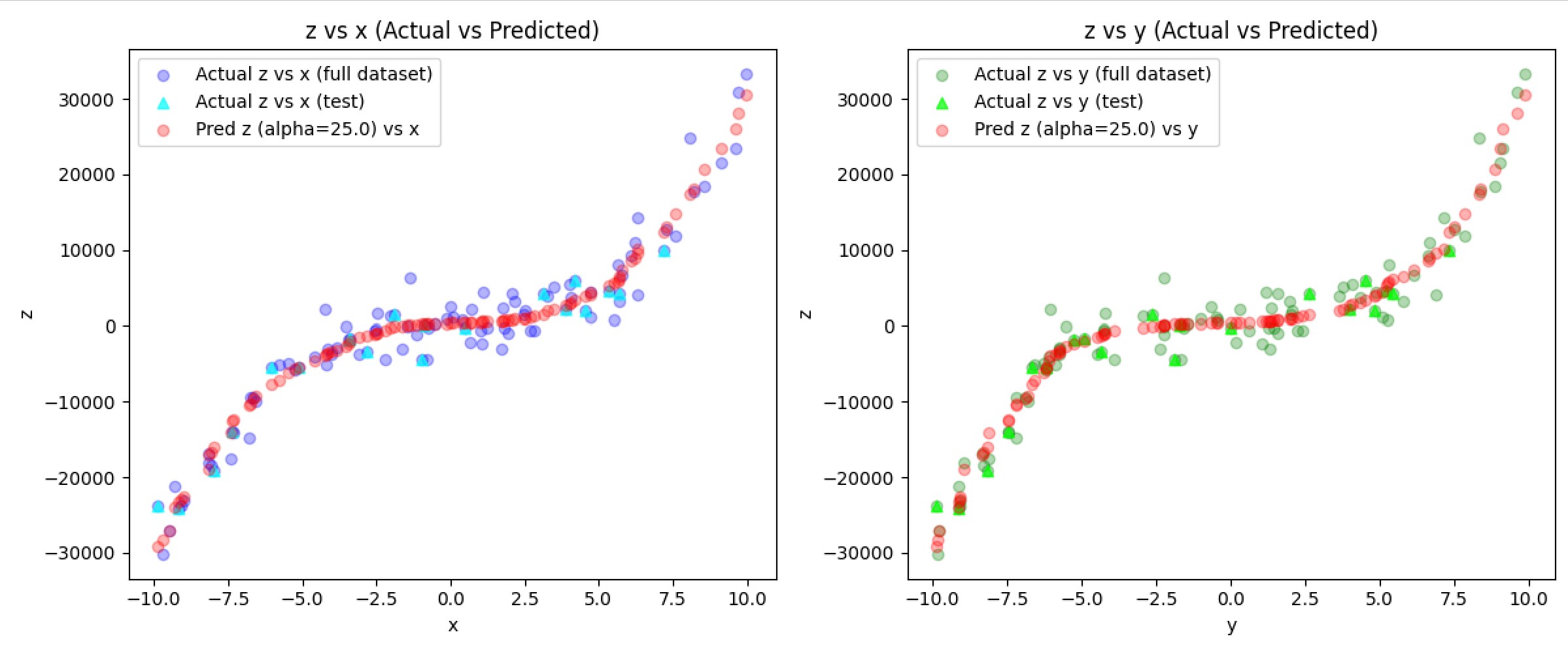
I thought alpha=25 provided a great balance between an overfit and underfit risk among all other cases I tested.

Training and Testing

I trained 5 models with degree 3 and alpha=25, each with a different random seed to account for variability. My trainingn splits were 80% train and 20% test. I picked the one with the lowest test MSE for simplicity. To double-check, I compared it against alpha=0, 10, 100, etc., and 25 still provided optimal results.

Since the z values were extremely large (in the billion) in comparison to the x and y values, I decided to use StandardScaler to normalize all values, then unscale predictions to match the original scale.

To prove it wasn’t a fluke, I made synthetic data mimicking the CSV files—100 samples with some extra large noise:

The model nailed it, balancing fit and generalization.

---

Unsupervised Learning: Gaussian Mixture Models

Task

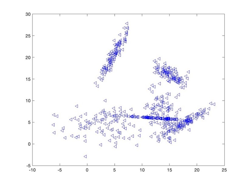
Given two datasets, A and B, the task was to identify the number of clusters (k), their means, and covariances using an unsupervised learning method. Additionally, I needed to determine if any clusters were repeated across the datasets.

• DatasetA
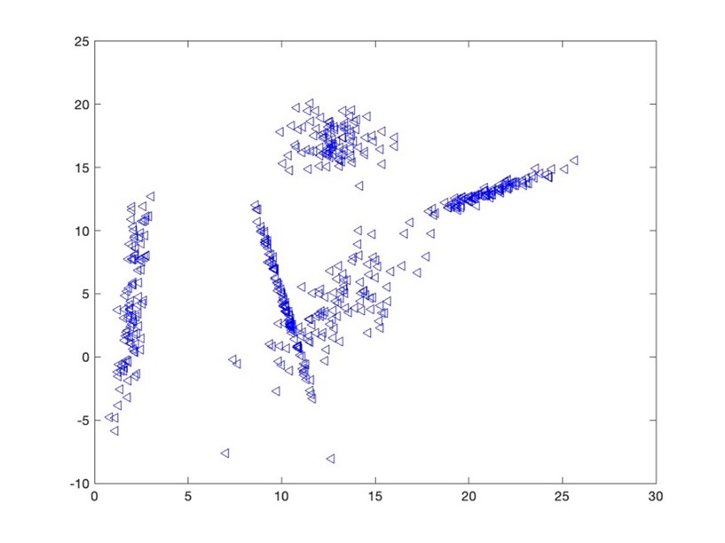
• DatasetB

Approach

I opted for Gaussian Mixture Models (GMM) since GMM is well-suited for ellipsoidal clusters. It’s also widely used in advanced applications, so I thought this could be a great way to learn about it.

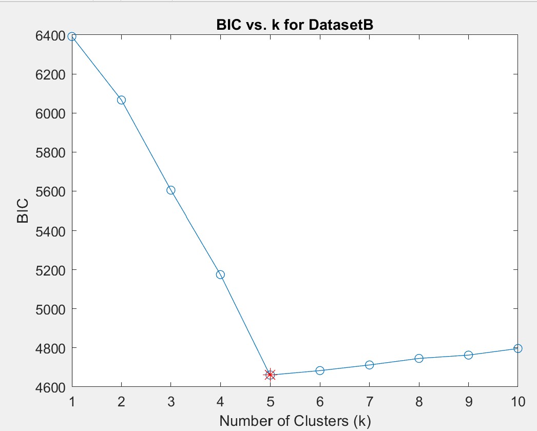
Using MATLAB, I applied the Bayesian Information Criterion (BIC) to determine k, testing values from 1 to 10. Before testing, I was predicting DatasetA should count for 6 clusters, and 5 clusters for DatasetB. There were much more overlap and spread-out clusters in DatasetA so I assumed it would be more difficult for the model to predict.

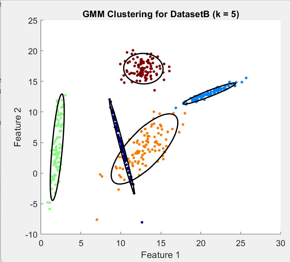
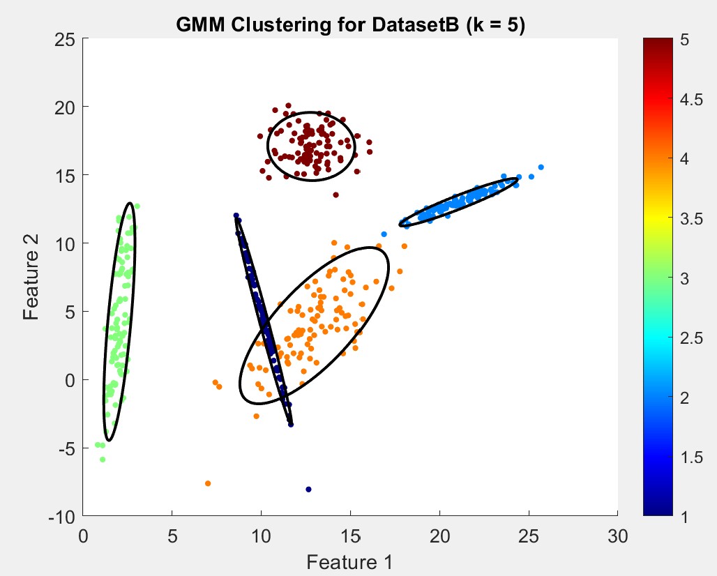
For DatasetB, BIC consistently indicated k=5, which aligned with the visualization:

DatasetA proved more challenging, with the BIC score fluctuating between k=6 and k=7:

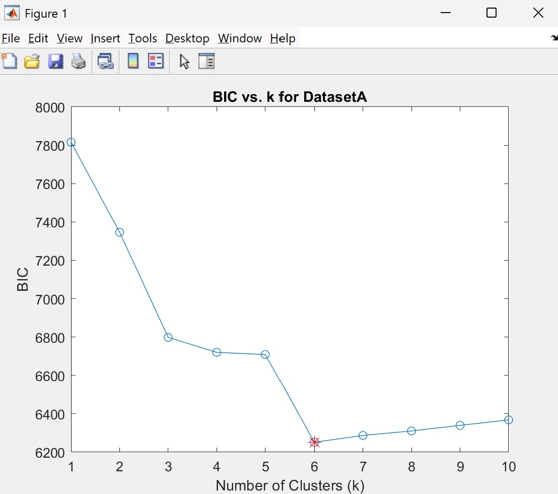
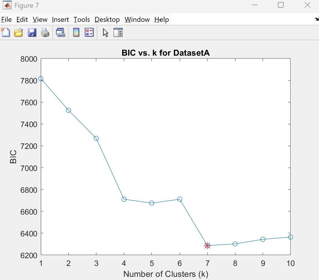
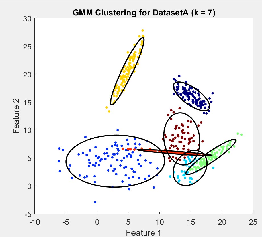
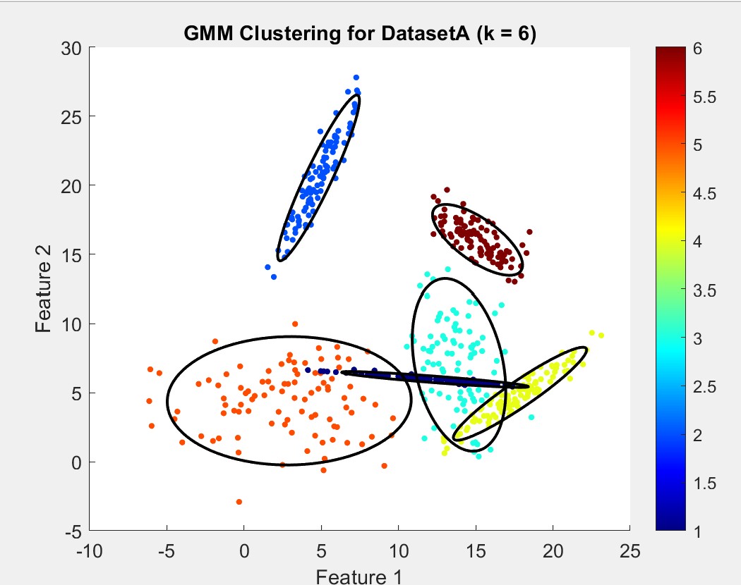
While k=7 occasionally appeared, it often over-segmented the data, leading me to select k=6 as the more reliable option based on both BIC and visual consistency. Most times it would split very obvious singular clusters in two. The following comparison displays the best version of k=7 I could obtain:

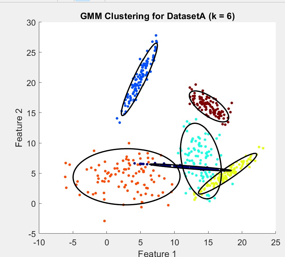
I was pretty satisified with choosing k=6 as my final cluster prediction as it was the safer option and more accurately represented the data in my opinion

Cluster Comparison

We can identify the clusters that may be repeated across datasets by calculating mean of each cluster and identifying which clusters have means that are similar or close to each other. It’s possible for two clusters to repeat across datasets, even if they don’t look exactly the same shape. This can happen because of different covariances for each clusters which modifies how enlarged and stretched the cluster looks.

To identify repeated clusters, I analyzed the means and covariances across datasets. Two pairs emerged as notable:

• DatasetA Cluster 3 (mean: 2.92, 4.42) and DatasetB Cluster 4 (mean: 2.04, 4.23)
• DatasetA Cluster 1 (mean: 12.36, 5.97) and DatasetB Cluster 1 (mean: 12.96, 3.95).

We have similar means and positions indicated by these numbers, however, their covariances also hint that they are reshaped and so may not be immediately recognizable in a scatter plot. Here are both scatter plots side-by-side, color is correspondant to cluster number:

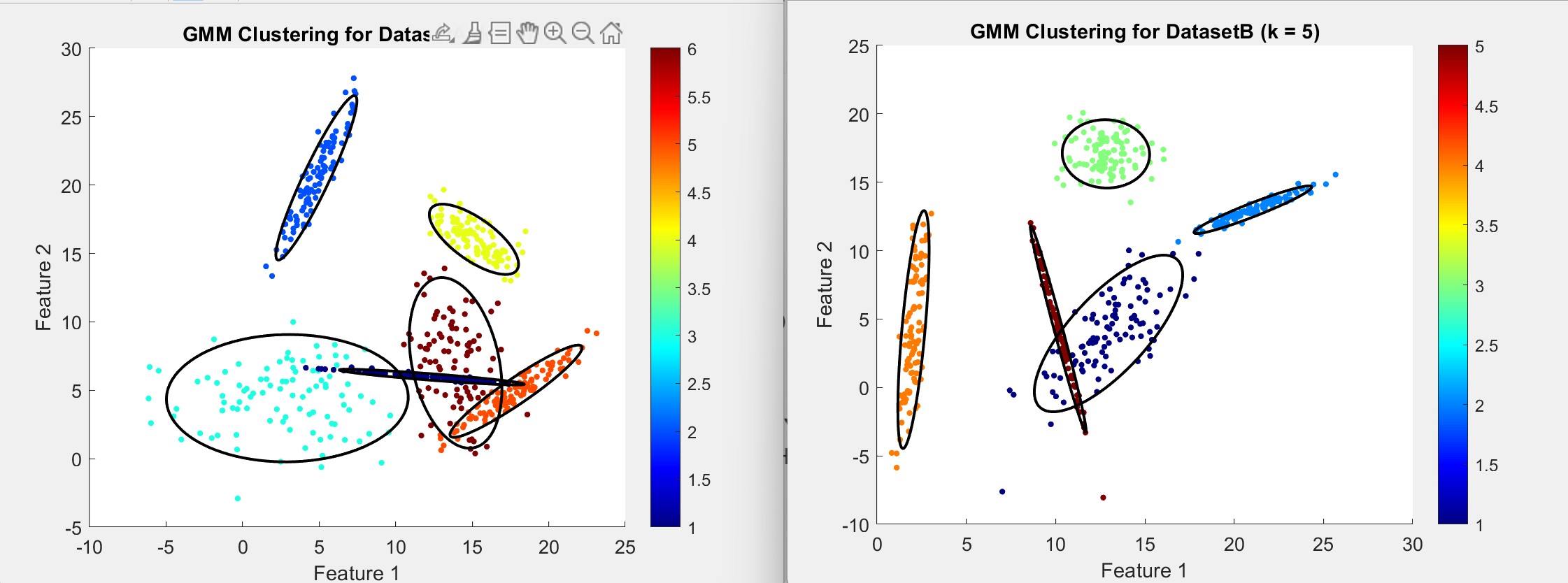
While the covariance differences highlight distinct cluster characteristics, the means were able to suggest repition for certain clusters across the datasets.

---

Gallery

---

Method Summary

PolyRidge

The cubic pattern in the data made Polynomial Regression a natural fit, and with only 50 samples, more complex methods like SVR or neural networks were probably impractical due to their tuning demands and computational needs. Ridge Regression addressed the noise effectively, with alpha=25 having a balance between overfitting (alpha=0) and underfitting (alpha=1000).

GMM

GMM was chosen over K-means for its ability to model probabilistic and non-spherical clusters, which matched the ellipsoidal shapes observed in the data. For DatasetA, k=6 prevented over-segmentation which was seen with k=7, while k=5 for DatasetB was consistently supported by BIC and visuals.

---

Conclusion

This was my first attempt at machine learning and I felt like I learned a lot. For supervised, PolyRidge with alpha=25 did great on following the cubic trend without overfitting. For unsupervised, GMM uncovered k=6 and k=5 clusters and taught me how means and covariances tell different stories. Figuring out the “why” behind my choices like regularization or BIC was the best part.